A quick step-by-step guide on adding checkboxes and a few ideas how to use them to manage and moderate your website content  

Did you know checkboxes are great not only for creating various to-do lists but also they can be a good alternative to copy-pasting while you work on your content? We gathered a few ideas on how you can use checkboxes for your SpreadSimple websites, but first let's cover how to add them to a Google Sheet.

How to add a checkbox to a Google Sheet

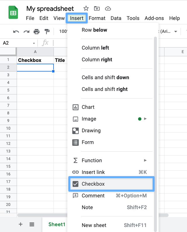
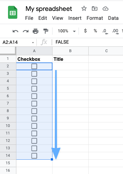
1. In your Google Sheet, click on the cell where you want to add a checkbox, then go to Insert and select Checkbox

To add checkboxes into the adjacent cells, grab the fill handle and then drag your checkboxes through the cells.

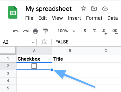
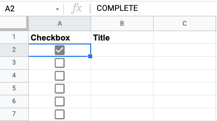
And you are good to go!

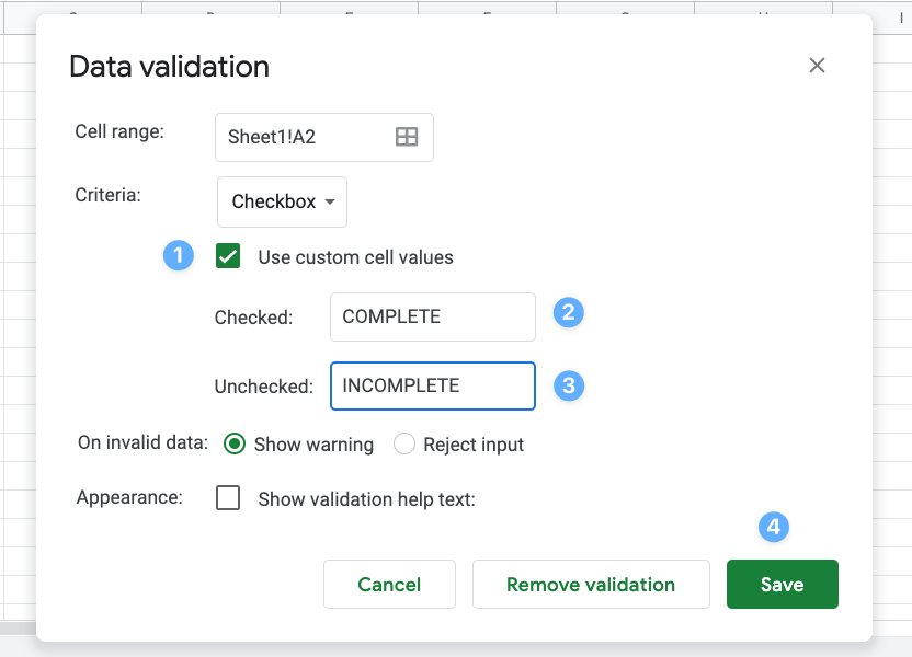
You can also change the default values (FALSE for empty cells, and TRUE for the checked ones). This is completely optional but we’ll be using this step later. If you want to add your custom values, right-click on the cell with a checkbox and select Data validation. On the Data validation window tick the Use custom cell values option, add your values into the corresponding fields, and save the changes.

Now your checkbox cells have your custom values

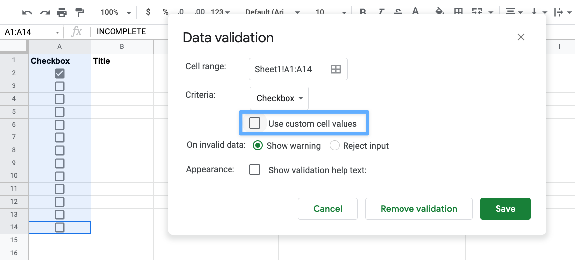
And you can always remove them by disabling the Use custom cell values on the Data validation window:

That's it! Now let's move to the most interesting part.

How you can use checkboxes for your SpreadSimple website

Here are a few ideas that hopefully you will find inspiring and useful for your projects.

Idea 1: Use checkboxes to select which items you want to highlight on the website.

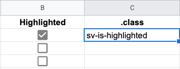
As you probably know, you can highlight some of your cards or listings on the site by using .sv-is-highlighted class:

This is how highlighted items look on the website

And this is how it looks on the source Sheet

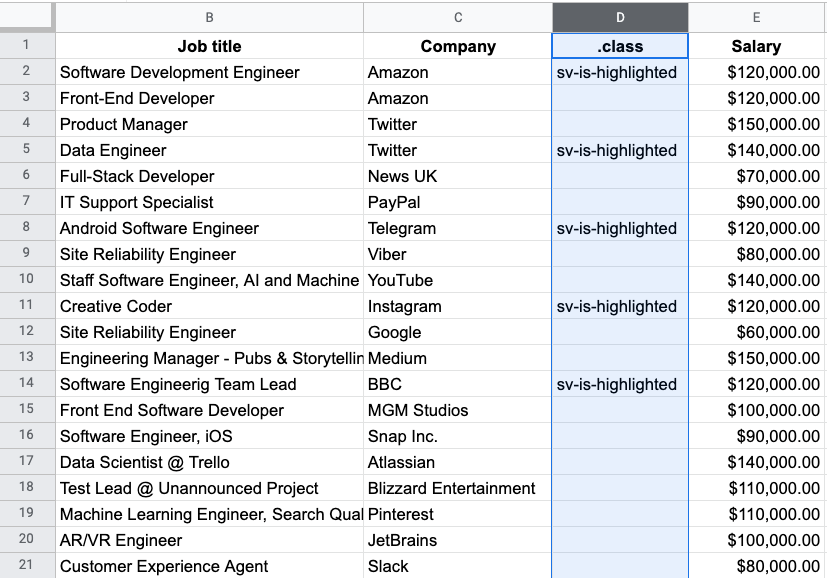
So to highlight an item, we need to make sure that the corresponding row has the required sv-is-highlighted value in a system column named .class.

But instead of copying and pasting sv-is-highlighted every time, why don’t we create one more column with checkboxes, and decide which items we want to highlight simply by ticking the boxes? All we need is two columns, checkboxes, and a Google Sheets =IF function.

Here’s what we do:

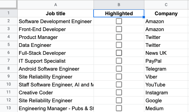
1. Create a new column in your Google Sheet and fill it with checkboxes.

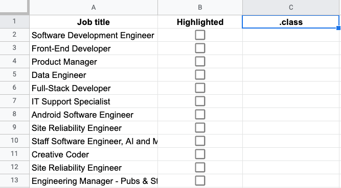
2. Then add another column and name it .class. This will be our system column containing the necessary values

The system column should be named .class only

3. In the system column (.class) we create =IF formula that will look like this: =IF(B2,"sv-is-highlighted","")

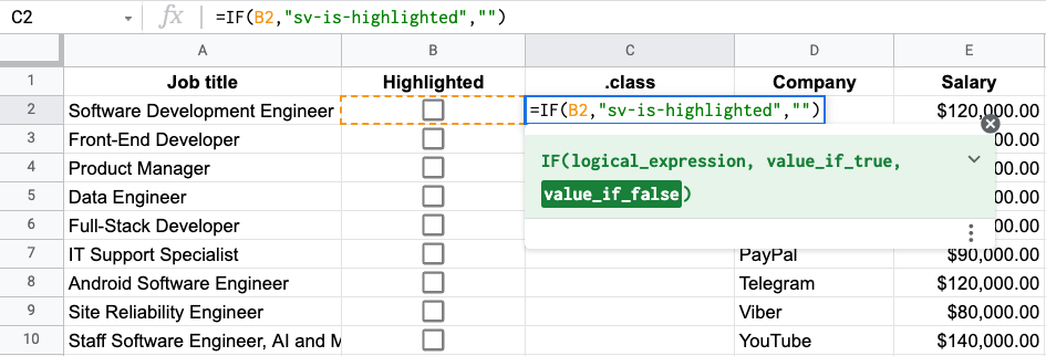
This means that if a checkbox in the Highlighted column is ticked, there will be the corresponding value in our .class column cell.

And we copy the formula by dragging the fill handle down the column.

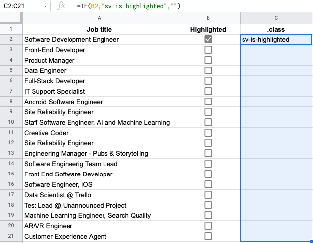
Now we can simply tick the box in a row to highlight that item on the website:

This was first approach, the "classic" one. And there's another way to use checkboxes for highlighting without =IF formula.
What we need to do here is to:

1. Create .class column.
2. Fill it with checkboxes.
3. Open Data validation field and select Use custom values option.
4. Add sv-is-highlighted to the Checked field.
5. Add any other value (for example -) to the Unchecked field.

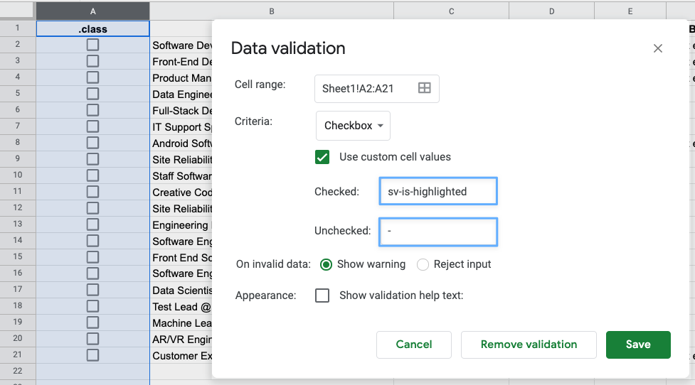
After that, if a box is checked, the cell will have the necessary value for system to highlight the corresponding item on the website.

And now let's move on to the second idea.

Idea 2: Combine checkboxes with the FILTER formula to moderate your website content

As you know, SpreadSimple displays all the data from a sheet, and sometimes you may want to choose which data to display on the website and which to hide. Of course, in such cases, you could manually add or delete certain rows from your source sheet, but a more convenient way to arrange that kind of content moderation is to use checkboxes alongside the =FILTER function.

What we need to do:

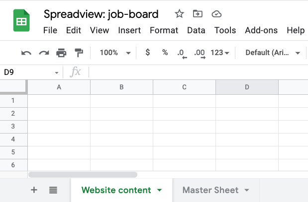
1. Create two sheets (tabs) in the same Google spreadsheet. One Sheet will be our “Master” Sheet and it will contain all the data. And the other Sheet will be a database for your SpreadSimple website and will have only filtered rows.

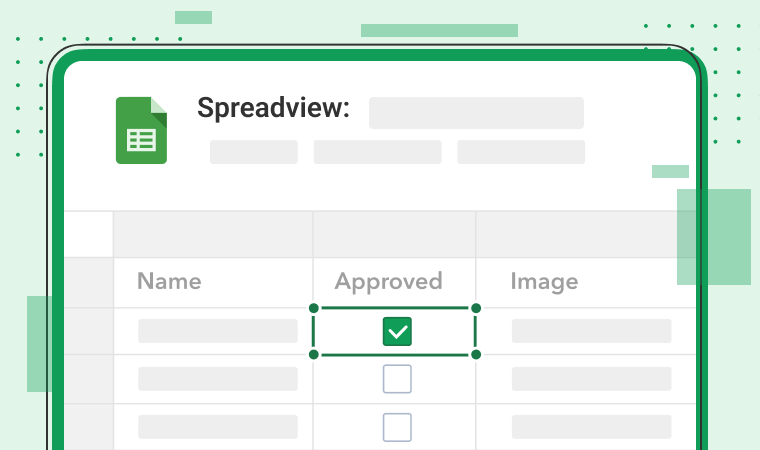
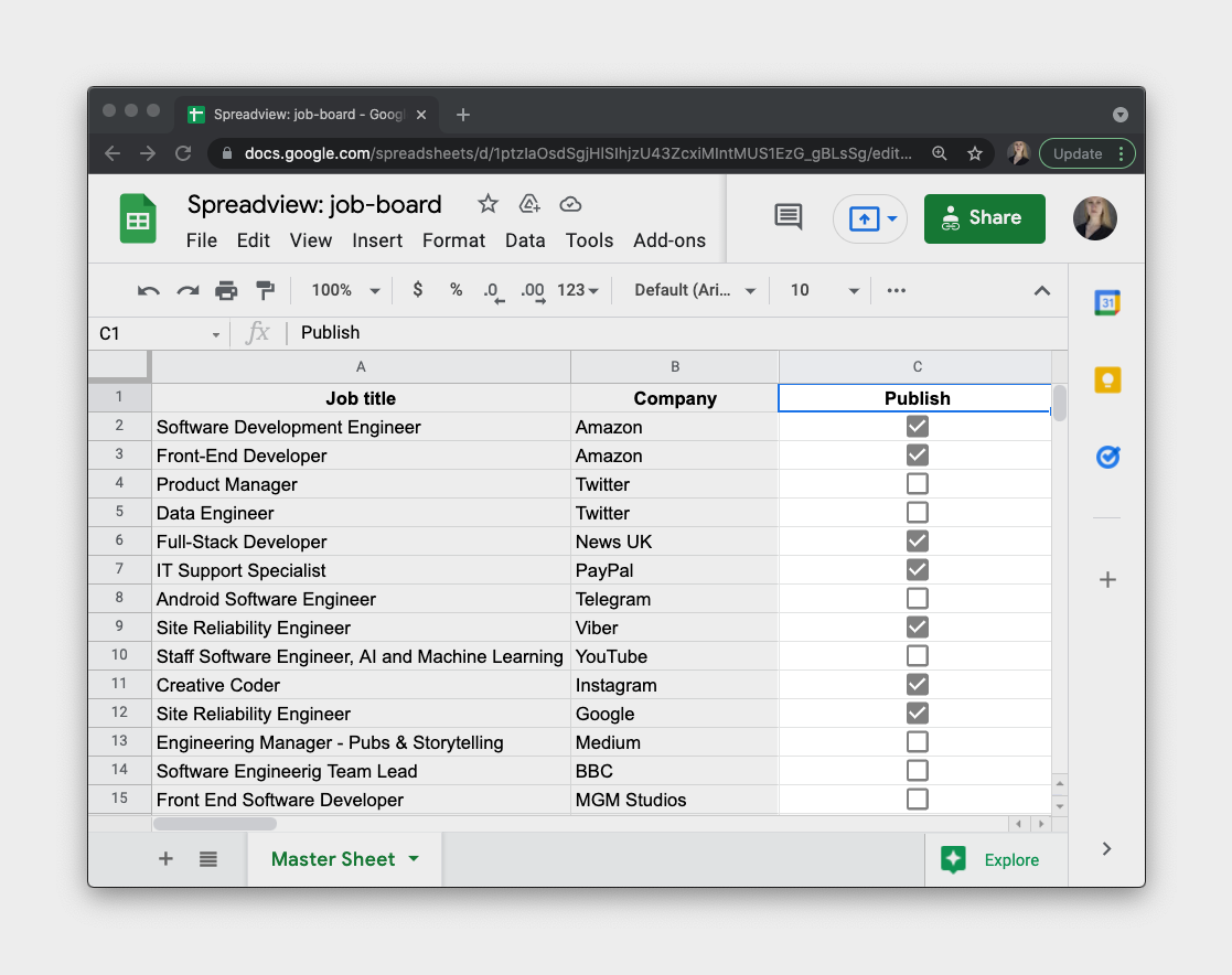
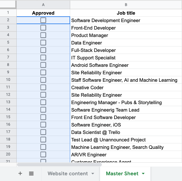
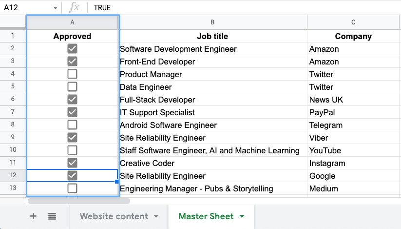
2. Now, in our “Master” Sheet, we create a column with checkboxes and let’s call it Approved

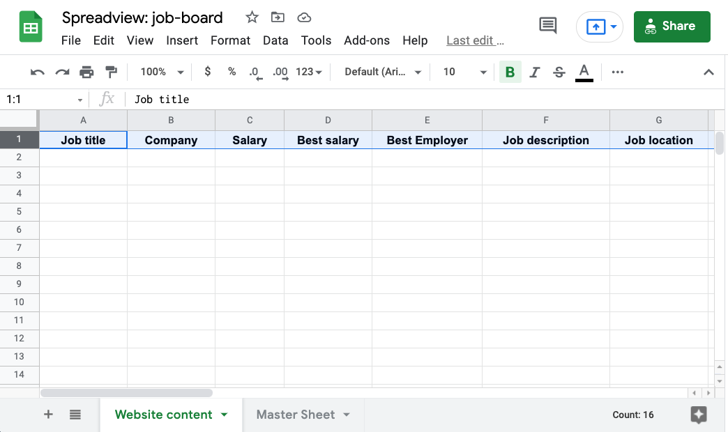
3. We copy the first row (column names) from Master Sheet to the sheet with website content. We can skip the Approved column as it’s not necessary to have it on the website content sheet

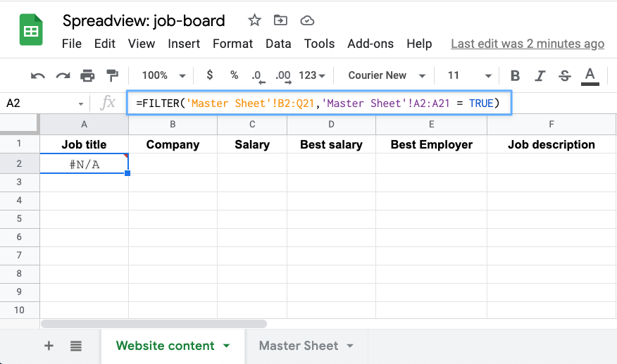
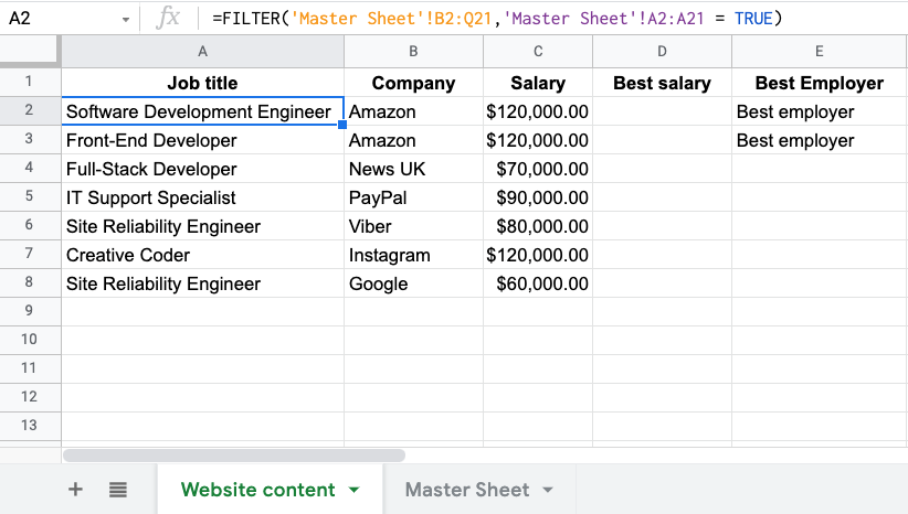
4. In cell A2 we create a Filter formula that includes the range of cells that will be copied from the Master Sheet if a certain condition is met: the checkbox in our Publish column is checked (the cell value is TRUE).
   Our formula looks like this:
   =FILTER('Master Sheet'!B2:Q21,'Master Sheet'!A2:A21 = TRUE)

5. And then we check all the listings that we want to display on our website…

… and get the filtered content just like this

This method can be great for cases when, for example, you are building a directory and you’re using a form to collect your users’ submissions. This way you can pre-moderate the content submitted via form before it appears on the website by just checking a box.

These were our ideas on using checkboxes for content management. Hope you find them helpful for your projects or they will inspire you and you'll find some use cases of your own.

---